Home Science Page Data Stream Momentum Directionals Root Beings The Experiment
In this first section we shall derive some very important theorems for our exploration. This will include the derivation of the Fraction and Denominator Series for square roots, i.e. the second order F&D Series.
Let us begin simply instead of universally. Let us begin with the derivation of the F&D Series for the individual number, 2. We shall sometimes refer to this number as the Root Number, or even the Number, indicated by capitals.
We begin with the following given.
Squaring both sides of the equation we get:
(A thought for later: We began with the positive square root of 2. Because of the squaring we could have also have started with the negative square root of 2.) Below is the simple expansion of step 2.
Some simple algebra yields:
Dividing by X+2,
Looking at Equation 1, we see that X also equals:
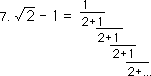
Replacing each X with the expression on the right in Equation 5 yields the following.
This is called an infinite continued fraction. We are going to be seeing a lot of these. Pietro Antonio Cataldi (1548? -1626) of Bologna created this derivation.
It is all very well to derive this expression for the square root of 2. But what does it mean? How is it computed? Infinite continued fractions don’t evoke any intuitive sense of magnitude. While we have the process of division to compute the comparative decimal value of ‘ordinary’ fractions, we have nothing comparable for these infinite continued fractions.
In order to compute the infinite continued fraction which equals x from step 7 above, we will break the fraction into smaller parts. These parts we will organize as a series. The limit of this series is √2- 1 = x. We will call the series, the Infinite Continued Fraction Series for √2, or the Fraction Series for √2, or simply the F Series for √2.
Let the first element of our series be the beginning, when there was nothing.
The second element is the infinite continued fraction abbreviated before the second fraction as shown below. The second term is an anticipation of the pattern to ensue.
The third element is abbreviated after the second term of the denominator as shown below.
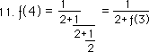
We continue the progression into the fourth element of the set.
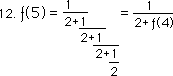
Continuing the progression into the fifth element, we see the emerging pattern.
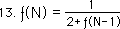
Generalizing our pattern, we can safely say that the Nth element of our set will be equal to the inverse of the quantity, 2 added to the prior member of the set, the N-1 element.
This is an iterative function, where each new member is based upon the one before. It is contextual rather than content based.
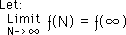
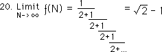
From Equation 7 above, we know that the limit of this F Series as N approaches ∞ is √2 -1. In order to deal with these infinite limits more efficiently let us first introduce a notational simplification that will be used throughout the paper.
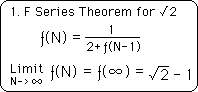
This allows us to express our first theorem, the F Series Theorem for √2, as it is stated below.
While this is our number 1 theorem, the First Theorem, as it were, it is only stated for a particular case for the time being. Throughout the course of this paper, this First Theorem shall be extended many times until it reaches complete universality for all positive rational roots. This is just the beginning.
Any real mathematician will immediately notice the lack of rigor in this presentation. The support for this First Theorem, upon which so must rests, is based upon pattern recognition. We must apologize for there is not a real mathematician among us. We are only after the truth. Once the pattern was sensed and recorded, it was computer tested to establish its validity. This is enough for us. If it is not enough for you, the Reader, then stop reading or prove it yourself, for there are many more patterns that have been recognized and computer-tested throughout this paper, that are called theorems. We are only after truth, not exactitude. If you, the Reader, are obsessed with exactitude to the exclusion of truth, this is not the paper for you. If however truth overwhelms exactitude in your mind set then read on, Brothers and Sisters of Life.
While the above series is based upon fractions, we would like to create a series based solely upon whole numbers.
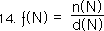
Let us create two new number series, the Numerator and Denominator Series, i.e. the N and D Series respectively. The Numerator Series contains all the numerators of the Fraction Series for √2, while the Denominator series contains all the denominators of the F Series for √2. The notation is shown below.
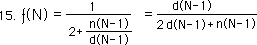
Replacing the N-1 element of the iterative expression for our F Series by our fractional definition in equation 13 and doing some elementary algebra we come up with:
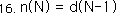
It is easy to see that the prior denominator is equal to the present numerator.
We use the equality of equation 16 to substitute d(N-2) for the n(N-1) expression in Equation #15. This is shown below.
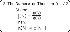
Notice that the N Series has completely dropped out of the expression for the F Series. Because the substitution of equation 16 allowed this to happen, we will call it our second theorem. We will call it the Numerator Theorem. It connects the Numerator series to the Denominator series in such a simple way that the N Series is completely neutralized and disappears. While it disappears, it leaves its mark in the intriguing second level of feedback, i.e. d(N-2).
Again the pattern was perceived and experimentally confirmed. This is the simplest manifestation of the Numerator Theorem.
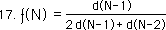
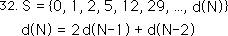
We can now see that the Nth element of the Denominator Series is given by the expression below, i.e. combining Equation 14 & 17.
Note that the D Series for the √2 is based upon two layers of feedback, not just one.
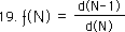
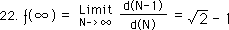
We see that our F Series can be written as a function of the D Series. In words, the Nth element of the F Series is the ratio of consecutive members of the D series.
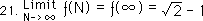
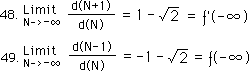
Before getting lost in symbols, let us remember where we are. The limit of our √2 series as N, the number of iterations, approaches infinity is shown below. This is merely an extension of equation 7, according to definition.
Simplifying Equation 20 with the ƒ(∞) notation, we introduced above,
We can replace our F Series by the ratio of the denominator series, from Equation 19.
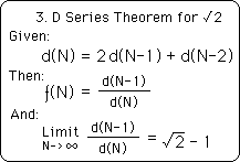
Now we can state our 3rd Theorem, the D Series Theorem for √2.
This theorem defines the connection between the F & D Series. The first statement defines the D Series. In this case the F Series is a function of the D Series. Under these conditions the Limit of the ratio of consecutive members of the D Series is √2 minus one. The original F Series was a function of itself, while this F Series is a function of the Denominator Series. The F Series is a series of fractions whose limit is the Root minus one, while the D Series are all whole numbers whose ratio generates the F Series. They are both the same F Series, but with different expressions.
Again this theorem is based upon the notoriously misleading pattern recognition. Again these theorems have been computer tested to establish their validity. (See the results in the chart at the back of the paper if interested.) Think of this style of mathematics as experimental mathematics, rather than purely analytical mathematics. The main difference that we are speaking of in this paper is that mathematical explorations are confirmed experimentally, i.e. through the computer, rather than searching diligently for an analytical proof of perceived patterns.
Notice that while the F Series is based upon only one layer of feedback that the D Series is based upon two layers of feedback. We’ll see much more of these feedback layers. We’ll call an equation with only one layer of feedback, a first order iterative equation. If the equation has two layers of feedback, we’ll call it a second order iterative equation. This will, of course, extend to third, fourth and fifth order iterative equations.
As we mentioned for the F Series Theorem above: this Third Theorem, the D Series Theorem, is only stated for a particular case for the time being. Throughout the course of this paper, this Second Theorem shall be extended many times until it reaches complete universality for all positive rational roots. As we stated before, this is just the beginning of the extension from the particular to the universal.
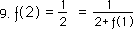
For curiosity’s sake, let us generate the D Series. From Equation 9 above, we get both the second element of both the numerator and denominator series'.
The second element of the numerator series is one.
The second element of the denominator series is two.
Applying Equation 16, we see that the first element of the series is one.
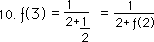
Now that we have the first two elements of the series we can generate the rest easily by applying Equation 18, in an iterative fashion.
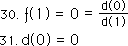
We also can find the zeroth element of our denominator by applying Equations 8 & 26.
Below is the set S, which is the set of numbers in the positive denominator series, generated by the definition immediately below.
The initial element is the zeroth element. The initial element is sometimes called the ‘seed’, because it gets the iterative process going. With first order iterative equations only one seed is needed. With our F Series equation, we let the seed equal zero, back in step 8. Because we were using the F series to generate the D Series, the seed had already been determined for the D Series. However if the D Series was to stand alone, it would need two seeds because it is a 2nd order iterative equation with two layers of feedback. In this case the two seeds were predetermined at 0 and 1 from the F Series. We will return to the importance of seeds soon.
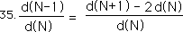
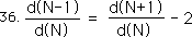
Performing simple algebra upon the definitional equation for the D Series, we get an equation that will allow us to generate a negative D series.
We add two to each of the members of the equation to get a more facile presentation.
Applying Equations 19 and 34 to the numerator of our equation.
Simplifying we find that the inverse ratios of our denominator series differ by two: A strange result. Most common series do not behave in such a fashion.
Remembering Equation 21, with notation.
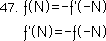
Let our inverse function be defined below.
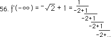
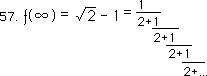
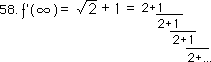
Applying Eq. 36 and 37 we come up with the following result. The infinite member of the inverse F Series equals √2 +1, while the infinite member of the regular F Series equals √2 -1.
Substituting -N for N in Equation 34, we get the following expression for generating the negative half of the denominator series.
The -1 element of the denominator series is generated easily and is the same as the first positive element.
The -2 element, or the 2nd element of the negative denominator series for √2, is the negative of the 2nd element of the positive denominator series.
Proceeding on with these contextual evaluations, we find that the odd elements of the negative denominator series are equal to the odd elements of the positive denominator series; while the even elements of the negative series are the negatives of the even elements in the positive denominator series.
Below is the whole denominator series for the √2, positive and negative sides. Notice that the absolute values of the elements are mirror images of each other. There is symmetry around the zeroth element.
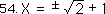
We see that the members of the negative D series alternate between negative and positive. To generate the negative √2 set by applying equation 19, we realize that all the members of this set will be negative because of this alternation. The members of the negative √2 set are the ratio of consecutive members of the negative denominator series, one positive, and the other negative. Furthermore because of the symmetry, the ratio for the negative series is reversed. Hence we arrive at these intriguing relationships.
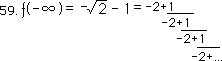
The elements of the positive √2 series are equal to the negative of the inverse function of the negative √2 series. The alternate is also true. Taking both of these expressions to negative infinity, we come up with the following results.
Let us look at another perspective, suggested above, that our derivation implies two roots, positive and negative. Let us start by assuming that X-1 = √2 rather than X+1, as in Equation 1.
We follow the same steps coming up with the negative result.
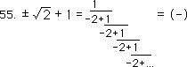
Looking at Equation 50 we realize that both roots are implied.
Looking at the positive expansion, we see that the result must be negative. Hence we realize that one root is derived by the positive expansion as N approaches positive infinity, while the other root is derived by the negative expansion as N approaches negative infinity.
Applying Equations 47 with notation, we come up with the following four equations.
Notice that to invert these infinite continued fractions it is only necessary to take the top off. This only works on the infinite continued fractions that are consistent in expansion. We will see later on that it only applies to square roots and rational numbers.
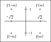
These four results generate a square of numbers. This is expressed below.
This graph is based upon the following equation.
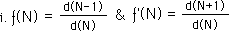
The F Series for √2 and its inverse, the F’ Series, are defined by the D Series as follows.
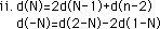
The positive and negative denominator series are generated by the following equations.
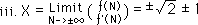
X equals the limit of the √2 series and its inverse, taken to positive and negative infinity. These are the four points in the square graph.
For the New-ager within us, this inherently balanced polarity is very exciting. We are thinking yin-yang and the in-between of Tai chi. We expect to find this same polarity extended to the Higher levels. Instead, we shall find that it is far more complicated than that.